Emerging Technologies in Research: Google Apps and SPSS
- Introduction
- Statistics
- Variable
- Measurement
- Measurement Scales
- Descriptive Statistics
- Boxwhisker Diagram
- Regression Analysis
- Simple Linear Regression
- Multiple Linear Regression
- Polynomial Regression Analysis
- Analysis of Variance (ANOVA)
- Analysis of Covariance (ANCOVA)
- Correlation Analysis
- Simple Correlation Analysis
- Partial Correlation Analysis
- Multiple Correlation Analysis
- Completely Randomized Design (CRD)
- Randomized Complete Block Design (RCBD)
- Latin Square Design
Introduction

alt text
Statistics
- Statistics deals with uncertainty & variability
- Statistics turns data into information
- Data -> Information -> Knowledge -> Wisdom
- Statistics is the interpretation of Science
- Statistics is the Art & Science of learning from data

Variable
- Characteristic that may vary from individual to individual
Measurement
- Process of assigning numbers or labels to objects or states in accordance with logically accepted rules
Measurement Scales
- Nominal Scale: Obersvations may be classified into mutually exclusive & exhaustive categories
- Ordinal Scale: Obersvations may be ranked
- Interval Scale: Difference between obersvations is meaningful
- Ratio Scale: Ratio between obersvations is meaningful & true zero point
Descriptive Statistics
- No of observations
- Measures of Central Tendency
- Measures of Dispersion
- Measures of Skewness
- Measures of Kurtosis
Example
| Fertilizer (Kg/acre) | Production (Bushels/acre) |
|---|---|
| 100 | 70 |
| 200 | 70 |
| 400 | 80 |
| 500 | 100 |

Analyze > Descriptive Statistics > Descriptives …


Boxwhisker Diagram
- Pictorial display of five number summary (Minimum, Q1, Q2, Q3 and Maximum)
Example
| Yield | Variety |
|---|---|
| 5 | V1 |
| 6 | V1 |
| 7 | V1 |
| 15 | V2 |
| 16 | V2 |
| 17 | V2 |

Graphs > Legacy Dialogs > Scatter/Boxplot …


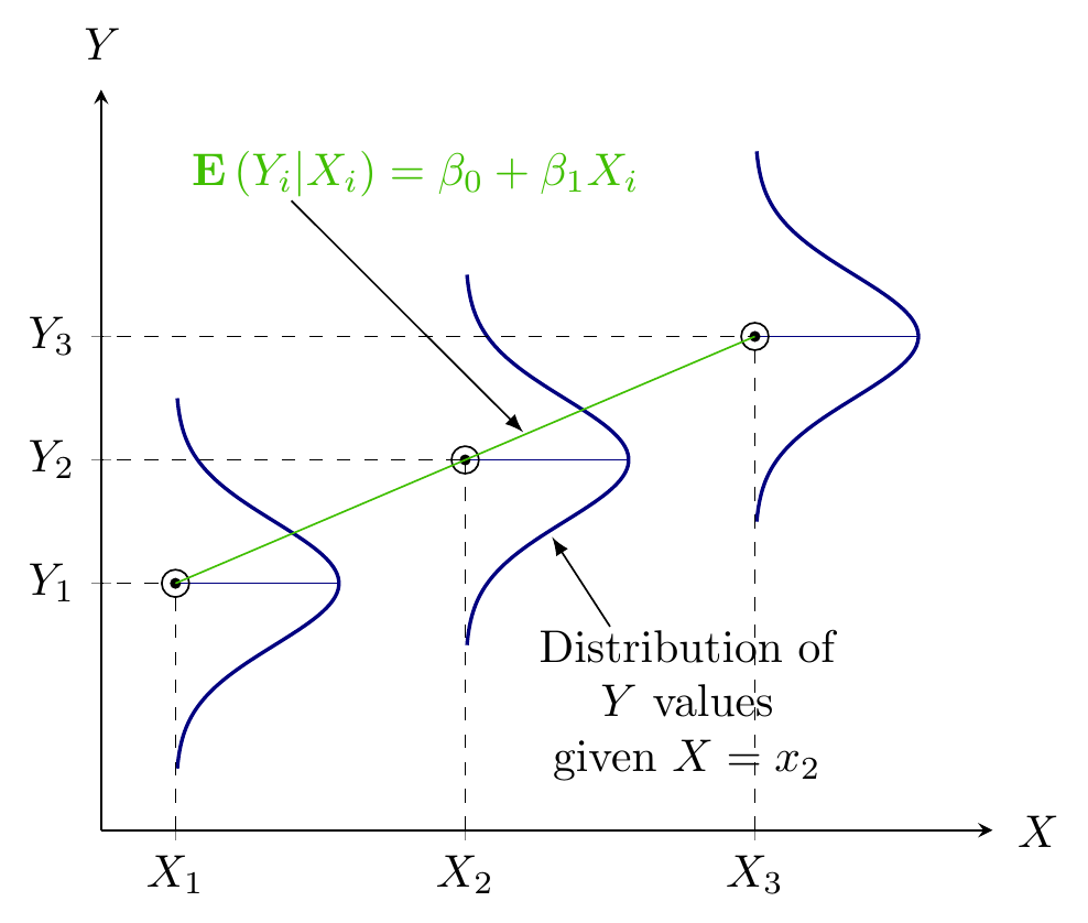
Regression Analysis
- Quantifying dependency of a normal response on quantitative explanatory variable(s)
alt text
Simple Linear Regression
- Quantifying dependency of a normal response on a quantitative explanatory variable
Example
| Fertilizer (Kg/acre) | Production (Bushels/acre) |
|---|---|
| 100 | 70 |
| 200 | 70 |
| 400 | 80 |
| 500 | 100 |

Graphs > Legacy Dialogs > Scatter/Dot …


Analyze > Regression > Linear …


Exercise
| Fertilizer | Yield |
|---|---|
| 0.3 | 10 |
| 0.6 | 15 |
| 0.9 | 30 |
| 1.2 | 35 |
| 1.5 | 25 |
| 1.8 | 30 |
| 2.1 | 50 |
| 2.4 | 45 |
Exercise
| Weekly Income ($) | Weekly Expenditures ($) |
|---|---|
| 80 | 70 |
| 100 | 65 |
| 120 | 90 |
| 140 | 95 |
| 160 | 110 |
| 180 | 115 |
| 200 | 120 |
| 220 | 140 |
| 240 | 155 |
| 260 | 150 |
Multiple Linear Regression
- Quantifying dependency of a normal response on two or more quantitative explanatory variables
Example
| Fertilizer (Kg) | Rainfall (mm) | Yield (Kg) |
|---|---|---|
| 100 | 10 | 40 |
| 200 | 20 | 50 |
| 300 | 10 | 50 |
| 400 | 30 | 70 |
| 500 | 20 | 65 |
| 600 | 20 | 65 |
| 700 | 30 | 80 |

Analyze > Regression > Linear …


Polynomial Regression Analysis
- Quantifying non-linear dependency of a normal response on quantitative explanatory variable(s)
Example
An experiment was conducted to evaluate the effects of different levels of nitrogen. Three levels of nitrogen: 0, 10 and 20 grams per plot were used in the experiment. Each treatment was replicated twice and data is given below:
| Nitrogen | Yield |
|---|---|
| 0 | 5 |
| 0 | 7 |
| 10 | 15 |
| 10 | 17 |
| 20 | 9 |
| 20 | 11 |
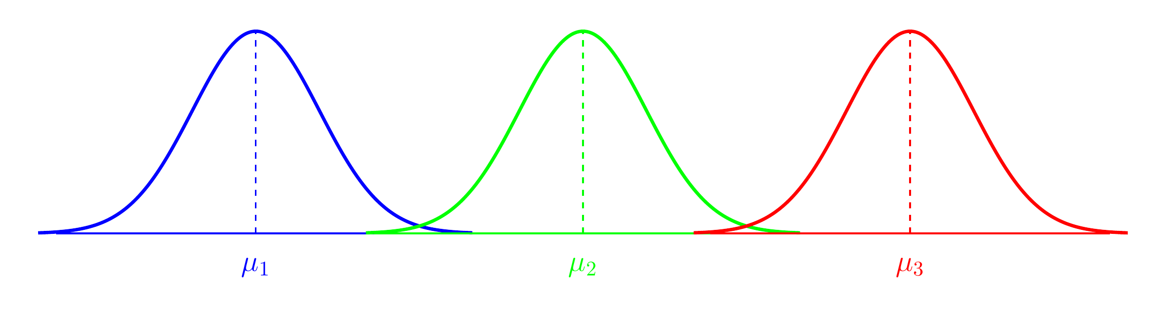
Analysis of Variance (ANOVA)
- Comparing means of Normal dependent variable for levels of different factor(s)
alt text
Example
| Yield | Variety |
|---|---|
| 5 | V1 |
| 6 | V1 |
| 7 | V1 |
| 15 | V2 |
| 16 | V2 |
| 17 | V2 |

General Linear Model > Univariate …


Exercise
| Yield | Variety |
|---|---|
| 5 | V1 |
| 7 | V1 |
| 15 | V2 |
| 17 | V2 |
| 17 | V3 |
| 19 | V3 |
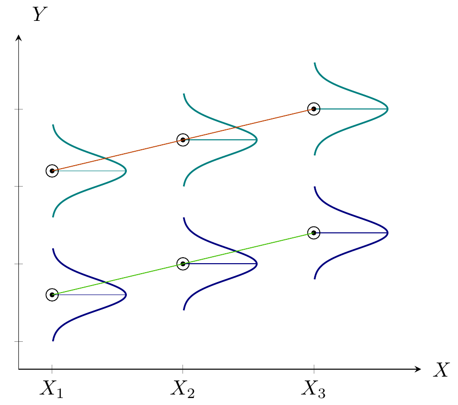
Analysis of Covariance (ANCOVA)
- Quantifying dependency of a normal response on quantitative explanatory variable(s)
- Comparing means of Normal dependent variable for levels of different factor(s)
alt text
Example
| Yield | Fert | Variety |
|---|---|---|
| 51 | 80 | V1 |
| 52 | 80 | V1 |
| 53 | 90 | V1 |
| 54 | 90 | V1 |
| 56 | 100 | V1 |
| 57 | 100 | V1 |
| 55 | 80 | V2 |
| 56 | 80 | V2 |
| 58 | 90 | V2 |
| 59 | 90 | V2 |
| 62 | 100 | V2 |
| 63 | 100 | V2 |
Same intercepts but different slopes
Different intercepts and different slopes
Correlation Analysis
- Linear Relationship between Quantitative Variables
Simple Correlation Analysis
- Linear Relationship between Two Quantitative Variables
- \(\left(X_{1},X_{2}\right)\)
Example
| Sparrow Wing length (cm) | Sparrow Tail length (cm) |
|---|---|
| 10.4 | 7.4 |
| 10.8 | 7.6 |
| 11.1 | 7.9 |
| 10.2 | 7.2 |
| 10.3 | 7.4 |
| 10.2 | 7.1 |
| 10.7 | 7.4 |
| 10.5 | 7.2 |
| 10.8 | 7.8 |
| 11.2 | 7.7 |
| 10.6 | 7.8 |
| 11.4 | 8.3 |

Analyze > Correlate > Bivariate …


Partial Correlation Analysis
- Linear Relationship between Quantitative Variables while holding/keeping all other constants
- \(\left(X_{1},X_{2}\right)|X_{3}\)
Example
| Leaf Area (cm^2) | Leaf Moisture (%) | Total Shoot Length (cm) |
|---|---|---|
| 72 | 80 | 307 |
| 174 | 75 | 529 |
| 116 | 81 | 632 |
| 78 | 83 | 527 |
| 134 | 79 | 442 |
| 95 | 81 | 525 |
| 113 | 80 | 481 |
| 98 | 81 | 710 |
| 148 | 74 | 422 |
| 42 | 78 | 345 |

Analyze > Correlate > Partial …


Multiple Correlation Analysis
- Linear Relationship between a Quantitative Variable and set of other Quantitative Variables
- \(\left(X_{1},\left[X_{2},X_{3}\right]\right)\)
Example
| Leaf Area (cm^2) | Leaf Moisture (%) | Total Shoot Length (cm) |
|---|---|---|
| 72 | 80 | 307 |
| 174 | 75 | 529 |
| 116 | 81 | 632 |
| 78 | 83 | 527 |
| 134 | 79 | 442 |
| 95 | 81 | 525 |
| 113 | 80 | 481 |
| 98 | 81 | 710 |
| 148 | 74 | 422 |
| 42 | 78 | 345 |
Completely Randomized Design (CRD)
- Used when experimental material is homogeneous
Example
The following table shows some of the results of an experiment on the effects of applications of sulphur in reducing scab disease of potatoes. The object in applying sulphur is to increase the acidity of the soil, since scab does not thrive in very acid soil. In addition to untreated plots which serve as a control, 3 amounts of dressing were compared—300, 600, and 900 lb. per acre. Both a fall and a spring application of each amount was tested, so that in all there were seven distinct treatments. The sulphur was spread by hand on the surface of the soil, and then diced into a depth of about 4 inches. The quantity to be analyzed is the “scab index”. That is roughly speaking, the percentage of the surface area of the potato that is infected with scab. It is obtained by examining 100 potatoes at random from each plot, grading each potato on a scale from 0 to 100% infected, and taking the average.
Randomized Complete Block Design (RCBD)
- Used when experimental material is heterogenous in one direction
Example
Yield : Yield of barley, SoilType : Soil Type, and Trt : 5 sources and a control
Latin Square Design
- Used when experimental material is heterogenous in two perpendicular directions
Example
The following table shows the field layout and yield of a 5×5 Latin square experiment on the effect of spacing on yield of millet plants. Five levels of spacing were used. The data on yield (grams/plot) was recorded and is given below: